Statistical Mechanics, Part 4

[This blog post is part of two series. The first series, titled Statistical Mechanics, is a series of lessons that I have developed to illustrate how curriculum and instruction can be designed to encourage vertical learning. We start by drilling down from our understanding of diffusion to develop a dynamic model of diffusion grounded in random particle motion using statistical mechanics. We then build on top of this foundation to construct deeper understandings of fluid flow, heat transfer, and electrical circuits. You can navigate through the lessons in this series using the links below. These lessons are then part of a larger series, Defining Vertical Learning.]

Part 1  |  Part 2  |  Part 3  |  Part 4  |  Part 5  |  Part 6  |  Part 7  |  Summary

Applying Statistical Mechanics to Model Dynamic Systems

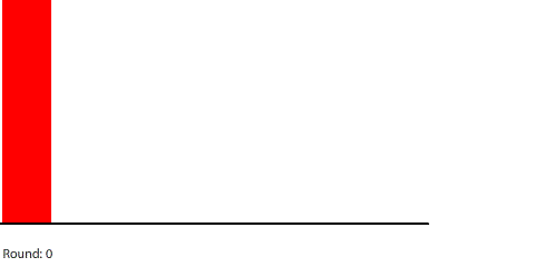
If all we know is that diffusion is the flow of particles from regions of high concentration to regions of low concentration, then we can predict the state of a pipe with red dye in it after it has reached equilibrium, but not much else. We have no sense of how long it takes for a system to reach equilibrium or what it looks like before that happens. But if we model diffusion with randomly moving pennies, we can observe diffusion as a dynamic process that occurs over time.

Diffusion in a 4-region pipe

Diffusion in a 6-region pipe

Diffusion in a 8-region pipe

For example, we can see that the rate of diffusion decelerates over time and that the time it takes to reach equilibrium grows longer as the pipe grows longer. I was curious about the relationship between pipe length and time to reach equilibrium, so I collected some data:

Rounds to reach equilibrium (±10%)

When I was conducting this investigation, I realized that I couldn’t count the number of rounds it took for the system to reach equilibrium. Because the rate of diffusion decelerates as the system approaches equilibrium, it’s hard to say when the system has actually gotten there. Instead, I counted the number of rounds it took for every region in the system to be within ±10% of the concentration the system will have when it does reach equilibrium.

One of the fun things to do when simulating a system is to try to create the same system in real-life to test and calibrate the model. It would be interesting to see if the concentration profile we see when we simulate diffusion in a pipe matches what we see in reality. I have been wondering if it is possible to use a camera to record dye diffusing in a clear pipe, and then to estimate concentration over time using color. Then, if the model is a reasonable approximation, you can try to figure out how long a round is in seconds or how wide a region is in centimeters.

It is important to demonstrate that the model reflects reality, otherwise the insights we gain from designing and running simulations won’t transfer to the physical world and we won’t be grounding our understanding at all. Our simulations don’t have to be completely accurate, but they do have to be accurate enough so that we can start to learn and explain why certain phenomena happen.

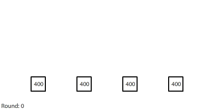
A block of 400 pennies dissolving

For example, here is a simulation of a block of solid red dye dissolving in water. The block of red dye is made up of 400 pennies in the solid state. When this block of red dye hits the water in region 1, it begins to dissolve as pennies leave the solid state and enter the water. The solid red dye continues to dissolve until there are 200 pennies in region 1. At that point, region 1 is “saturated.” If the number of pennies in region 1 dips below 200, then more pennies will dissolve to make up the difference until the block of solid red dye is completely gone. In this simulation, the block of red dye disappears after 4 rounds.

A block of 800 pennies dissolving

What happens if the block of solid red dye is made up of 800 pennies? It takes 21 rounds for the block to disappear, which is over five times longer. It takes 1 round for the first 200 pennies to dissolve, 3 rounds for the next 200, 7 rounds for the third 200, and then 10 rounds for the last 200. Why does it take longer for the dye to dissolve later? What would happen if the block of solid red dye was made up of 1600 pennies? It may not actually take five times as long for twice as much red dye to dissolve if we conduct this experiment in the real world, but it does take longer and we can figure out why by studying the simulation. In fact, we can learn a lot just be designing the simulation and trying to make it more accurate.

A 4-region block dissolving in two dimensions

Our simulation was only in one dimension, and the block did not get smaller as it dissolved. Here is a 4-region block dissolving in two dimensions. This time, a region is saturated when it has 100 pennies. The top two regions dissolve after 11 rounds, and the whole block is gone after 21 rounds. Why do the top two regions dissolve faster?

Four 1-region blocks dissolving in two dimensions

If we simulate four 1-region blocks dissolving in two dimensions, the blocks dissolve only after 7 rounds. Why do four individual blocks dissolve faster than four blocks stacked together? And even though all four blocks disappear after 7 rounds, the two outer blocks do dissolve slightly faster than the two inner blocks.

By modeling the system with randomly moving pennies and observing what happens over time, we gain a deeper understanding of the system than if we simply know what the system looks like when it has finally reached equilibrium.


Part 1  |  Part 2  |  Part 3  |  Part 4  |  Part 5  |  Part 6  |  Part 7  |  Summary