Statistical Mechanics, Part 5

[This blog post is part of two series. The first series, titled Statistical Mechanics, is a series of lessons that I have developed to illustrate how curriculum and instruction can be designed to encourage vertical learning. We start by drilling down from our understanding of diffusion to develop a dynamic model of diffusion grounded in random particle motion using statistical mechanics. We then build on top of this foundation to construct deeper understandings of fluid flow, heat transfer, and electrical circuits. You can navigate through the lessons in this series using the links below. These lessons are then part of a larger series, Defining Vertical Learning.]

Part 1  |  Part 2  |  Part 3  |  Part 4  |  Part 5  |  Part 6  |  Part 7  |  Summary

Applying Statistical Mechanics to Model Dynamic Systems with Net Flow down Gradients

When a region of high concentration is next to a region of low concentration, there is a net flow of particles. This net flow does not occur because something is causing the particles to flow in a particular direction. The particles are still moving randomly, but more particles are moving from high to low concentration than from low to high concentration simply because there are more particles on the high concentration side.

There is a net flow of 8 pennies to the right
when half of the 38 pennies move to the right
and half of the 22 pennies move to the left.

The net flow between two regions is proportional to the difference in their concentrations. In our example, that difference is 16 pennies (38 − 22 = 16), which gives us a net flow of 8 pennies. If the concentration difference between two regions was 24 pennies (34 − 10), then the net flow would be 12 pennies.

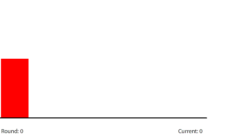
There is a net flow of 12 pennies to the left
when half of the 10 pennies move to the right
and half of the 34 pennies move to the left.

A change in concentration over distance (across regions) is known as a concentration gradient. You can think of the gradient as a hill. There is a net flow of particles down the concentration gradient. The “steeper” the gradient, the greater the net flow.

Diffusion is not the only process generated by random particle motion creating a net flow down a gradient. An electrochemical cell inside of a battery contains an anode (negative terminal) and a cathode (positive terminal). The way a battery works is that a chemical reaction produces electrons at the anode and another chemical reaction removes electrons at the cathode. When a wire connects the anode to the cathode, electrons flow and an electric current is generated within an electrical circuit.

We are going to simulate this electrical circuit by making region 1 the anode and region 7 the cathode. There is a chemical reaction producing electrons at the anode that will keep the number of pennies in region 1 at 240. There is a chemical reaction removing electrons at the cathode, so any pennies that arrive at region 7 will be removed from the system. The 240-penny difference between the anode and the cathode is the potential difference across the circuit, and the net flow of pennies (electrons) through the system is the current. We will measure the current by counting the number of pennies removed at the cathode in each round.

A 7-region circuit with a 240-penny potential difference

By round 41, the system has reached a steady state where the number of pennies in each region does not change. If we actually count them, we can see that the number of pennies in each region drops by 40 going from left to right. At steady state, the 240-penny potential difference across the entire circuit is now divided evenly (240 ÷ 6 = 40) across the six control surfaces and seven regions. This results in a net flow of 20 pennies into each region from the left that is balanced by an equal net flow of 20 pennies out of each region to the right.

With a 40-penny difference between regions, the net
flow from region to region in each round is 20 pennies.

What happens if we reduce the potential difference across the circuit to 120 pennies or shorten the length of the circuit to five regions?

A 7-region circuit with a 120-penny potential difference

With a 20-penny difference between regions, the net
flow from region to region in each round is 10 pennies.

Reducing the potential difference across the entire circuit to 120 pennies reduces the potential difference between regions to 20 pennies (120 ÷ 6) at steady state. The potential gradient isn’t as steep and the current decreases to a net flow of 10 pennies per round.

A 5-region circuit with a 240-penny potential difference

With a 60-penny difference between regions, the net
flow from region to region in each round is 30 pennies.

Shortening the circuit to five regions means that the 240-penny potential difference will be divided evenly across four control surfaces at steady state. The potential gradient is steeper and the current increases to a net flow of 30 pennies per round.

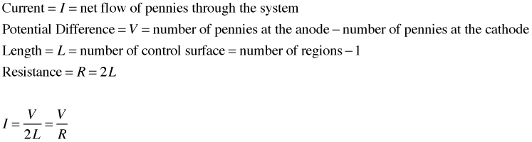
If we wanted to, we could develop a formula to calculate the current through a circuit given the potential difference across the circuit and the length of the circuit:

Then, if we define the resistance in the circuit as 2L, we have Ohm’s law:

We shouldn’t be surprised that electric currents and diffusion share certain basic features and can be described by similar models. After all, when you drill down to their local mechanisms, both processes are generated by random particle motion creating a net flow down a gradient. By building both processes on top of the same foundation, we strengthen that foundation and encourage learning to go vertical. A little bit later in this lesson, we will be extending our model to simulate two additional processes, fluid flow down a pressure gradient and heat transfer down a temperature gradient.


Part 1  |  Part 2  |  Part 3  |  Part 4  |  Part 5  |  Part 6  |  Part 7  |  Summary