Statistical Mechanics, Summary

[This blog post is part of two series. The first series, titled Statistical Mechanics, is a series of lessons that I have developed to illustrate how curriculum and instruction can be designed to encourage vertical learning. We start by drilling down from our understanding of diffusion to develop a dynamic model of diffusion grounded in random particle motion using statistical mechanics. We then build on top of this foundation to construct deeper understandings of fluid flow, heat transfer, and electrical circuits. You can navigate through the lessons in this series using the links below. These lessons are then part of a larger series, Defining Vertical Learning.]

Part 1  |  Part 2  |  Part 3  |  Part 4  |  Part 5  |  Part 6  |  Part 7  |  Summary

Summary

A mental model is our internal theory for how and why something works. We learn when we construct new mental models and revise old ones. Even when we read something in a textbook or hear something in a lecture, we don’t actually learn anything until we integrate it into a mental model.

New mental models are almost always naive. They are an initial attempt at trying to make sense of something. Mental models only become powerful and sophisticated once they have been applied repeatedly and revised over time to accommodate new data. We revise mental models when they don’t work reliably, we encounter edge cases, we want to broaden the contexts in which they can be applied, or we want to unify several separate models into one general model.

Ideally, we would be actively seeking opportunities to revise our mental models all the time because revising a mental model increases our level of understanding, and improving our ability to revise mental models increases our capacity to learn. But in reality, many of us shy away from revising mental models. We are often emotionally invested in the existing mental model, frightened of feeling destabilized after the existing mental model has been disrupted but before a revised model can take its place, and uncertain if the revised mental model will be any better.

Learning horizontally in silos

Our reluctance to revise our mental models is often compounded by the horizontal nature of traditional schooling. In schools, most learning happens in silos. Not just silos for subjects, but silos for topics within subjects. We learn something to pass a test, and then we instantly forget it. It’s actually a bit shocking when a teacher references something that you learned a few months ago as though you were suppose to remember it. Horizontal learning discourages us from investing the time and resources required to revise our mental models because we aren’t given the time and we are constantly asked to abandon what we were just building to start something new.

Learning vertically: gaining access through
an entry point and then branching up and out

But vertical learning is designed to encourage mental model revision. It challenges and supports us to construct better and better theories over time so that we can understand and do more. It does this by reducing the cost and increasing the benefits of revising a mental model. Starting at an easily accessible entry point, we feel capable and successful when we build on a theory and then find ourselves racing upward and outward on our own. This tips our risk/reward calculation in favor of revision, and helps us learn that we can survive brief periods of destabilization and gain confidence that our revised mental model will be worth the effort.

Modeling diffusion with randomly moving pennies makes diffusion more accessible along multiple dimensions. First, it makes diffusion more concrete. We can understand it on an intuitive level and apply our common sense to reason about it. Second, we don’t have to build a new foundation for it; we can build on top of an existing foundation, which saves time and minimizes the things we need to know. We are more willing to invest in a shared foundation because we know we can leverage it in many different ways.

Blocks of red dye dissolving in water

Third, simulating diffusion creates an immersive experience that stimulates our natural curiosity. It is hard to watch blocks of red dye dissolving in water and not think about what we are observing. When we see something, we look for patterns and want to make sense of it, even if we don’t care about it on a conscious level. That’s just how our brains are wired. Fourth, every simulation is also completely transparent. We can calculate the state of the simulation for any round, which means we can replay time and see and know everything that happens. This invites analysis. Because we can know, we want to know.

Diffusion is more accessible when we make it more concrete, immersive, and transparent, and build it on top of a shared foundation. In turn, this makes it easier, less risky, and less costly to revise our mental model of diffusion. We are much less willing to revise our mental models about something that we perceive as arcane and unknowable.

Vertical learning also works on the reward side, increasing the benefits when we do revise our mental models. For example, when simulating blocks of red dye dissolving in water, we can see that blocks A and B dissolve faster than blocks C and D, and we might theorize that happens because blocks A and B expose more surface area to the water.

Directions in which the four blocks dissolve

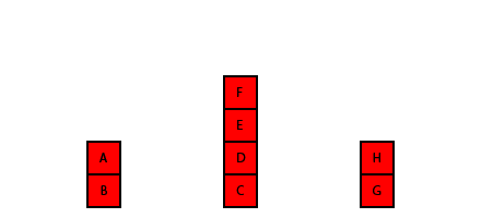
That’s a useful mental model, but it doesn’t work in all situations. If we separate the four blocks, blocks A and D dissolve faster than blocks B and C even though all four blocks expose the same amount of surface area to the water.

Four separate blocks of red dye dissolving in water

Concentration gradients in the water and
directions in which four separate blocks dissolve

To understand this new simulation, we need to revise our mental model to also think about the concentration gradients in the water. The blocks of red dye will dissolve faster where there is less red dye already in the water, and that is toward the left, right, and top edges of the water. From there, we can analyze and predict what will happen in other situations.

In what order will the blocks dissolve? Does it matter
how far apart the stacks are, or how wide or tall the water is?

While this problem may not be intrinsically relevant to students, it is far more interesting than what they typically work on. Imagine a sixth-grader breaking the problem down by sketching isoconcentration maps and estimating diffusion rates by how steep the gradients are. It feels powerful and the student feels successful. And it is a level of thinking that is accessible to all students because the model is concrete, immersive, and transparent, and it builds on top of a shared foundation.

When we extended our model to include solubility, I simply said that enough red dye will dissolve from a block to keep the region around the block saturated. That allowed us to model solubility at a macroscopic scale, but not on a molecular scale. Particles don’t know or care anything about saturation concentrations.

At a molecular scale, there is a probability that a particle in
the solid state will transition to the liquid state, and a probability
that a particle in the liquid state will transition to the solid state.

But if we decided to drill down and understand solubility at the molecular scale, then we could model red dye particles transitioning between the solid state and the liquid state along a surface using probabilities, and we could see how and why a system would reach a saturation concentration dynamically. By extending our model and the shared foundation it builds on, we would gain a deeper understanding of solubility and we would be able to solve complex problems where solubility and diffusion are integrated.

Similarly, we could extend our model to simulate reaction rates, since reaction rates are also driven by the probability that reactant particles collide. And from there, we could design and calculate reaction rates in a reaction chamber where reactants are introduced as solid blocks. This is something that I studied as a chemical engineer.

Vertical learning lowers the cost of revising our mental models by making the process easier and more accessible. It also increases the benefits of revising our mental models by enabling us to leverage those mental models to learn and understand more deeply, develop and apply higher-order thinking skills, and solve rich and complex problems. But the ultimate benefit is developing the skills and confidence we need to revise our mental models on our own in life. Because when we do that, we can do anything.


Part 1  |  Part 2  |  Part 3  |  Part 4  |  Part 5  |  Part 6  |  Part 7  |  Summary

Statistical Mechanics, Part 7

[This blog post is part of two series. The first series, titled Statistical Mechanics, is a series of lessons that I have developed to illustrate how curriculum and instruction can be designed to encourage vertical learning. We start by drilling down from our understanding of diffusion to develop a dynamic model of diffusion grounded in random particle motion using statistical mechanics. We then build on top of this foundation to construct deeper understandings of fluid flow, heat transfer, and electrical circuits. You can navigate through the lessons in this series using the links below. These lessons are then part of a larger series, Defining Vertical Learning.]

Part 1  |  Part 2  |  Part 3  |  Part 4  |  Part 5  |  Part 6  |  Part 7  |  Summary

Boundary Layers

So far we have applied our model to simulate the flow of solute particles in diffusion, the flow of electrons in an electrical circuit, and the flow of fluid through pipes. When analyzing diffusion and electrical circuits, we found that a net flow of particles was generated between regions when there was a difference in the number of particles in those regions, and that this behavior at the molecular scale resulted in behavior at the macroscopic scale that matches what we would expect to see in the real world.

There is a net flow of 8 pennies to the right
when half of the 38 pennies move to the right
and half of the 22 pennies move to the left.

A circuit with four resistors. Resistors B and C are in parallel.
The potential difference across the entire circuit is 1560 pennies.

If we were to release a gas in an empty container, we would expect to see it spread out just like our red dye did when we dropped it in water.

Red gas filling an empty box

Red dye diffusing in a glass of water

The major difference is that the red gas particles are moving randomly in a vacuum while the red dye particles are moving randomly through a solvent. We say that there is a net flow of red gas particles down a pressure gradient and there is a net flow of red dye particles down a concentration gradient, but at a molecular scale, there is no such thing as pressure or concentration. Pressure and concentration are measured at a macroscopic scale. At a molecular scale, all we have are particles moving randomly and colliding with one another.

If we simulate the two systems, the models look the same.

Red gas flowing and filling 8 regions

For diffusion, we could include solvent particles in our model. If pennies represent red dye particles, we could use nickels to represent water molecules. The nickels would also move randomly left and right, hopping from region to region. But since there are an equal number of nickels in each region, the net flow of water molecules between regions would be zero. The presence of the solvent particles do affect the time and distance scales in our simulation when we calibrate it against reality, but they don’t affect the simulation itself.

Red dye diffusing in water in 8 regions

If we connect one end of a hose to a pressurized tank of gas and let the gas vent out the other end into a vacuum, our simulation looks a lot like an electrical circuit.

Hose connected to a pressurized tank of gas
at one end and to a vacuum at the other end

Pressure and number of particles in an 8-region hose

The pressure and number of gas particles in region 1, where the hose is connected to the tank, is high. As we move down the hose and to the right, the pressure and the number of gas particles in each region drops, until both are zero at the end of the hose that is sitting in vacuum. The difference in the number of gas particles in each region generates a net flow of gas particles through the hose. If this were a spaceship in outer space, this net flow of gas particles would thrust the spaceship in the opposite direction.

Our model accurately describes fluid flow when the fluid is a gas, but not when it is a liquid. In a garden hose, there is a pressure drop from the start of the hose to the end of the hose which generates the flow of water, but there isn’t a corresponding drop in the number of water molecules in each region. This is because liquid water is relatively incompressible. Unlike a gas, doubling the pressure on a volume of liquid water does not compress the water and double its density.

At a macroscopic scale, gases and liquids both flow in the same way, which is why they are both classified as fluids. But on a molecular scale, they behave differently. You can still use our model to simulate the flow of liquids, but only if you abstract away the molecular view and think in terms of pressure.

The final kind of flow that we are going to simulate with our model is the flow of heat. To model heat transfer, we are going to use hot and cold particles. In this simulation, we have a tank with hot liquid particles on the left and cold liquid particles on the right.

Hot and cold particles mixing

Over time, the hot and cold particles mix. Because the particles are actually moving from region to region, we are simulating convection. However, the total number of particles in each region isn’t changing because all of the regions have the same number of particles and the net flow of total particles is zero.

Temperature gradient of the system as the hot and cold particles mix

Instead of graphing the number of hot and cold particles in a region over time, we can also graph the temperature. Temperature is a measure of the average kinetic energy of the particles in a region, so it is based on the ratio of hot to cold particles. Since the total number of particles in a region isn’t changing, the temperature graph looks just like a graph of the number of hot particles. In heat transfer, heat flows down a temperature gradient.

On the surface, it seems unlikely that we would be able to simulate heat transfer through conduction using our model because, in conduction, heat is transferred through collisions and not the net movement of particles. Our entire model is grounded on random particle motion.

Heat transfer through convection

If we are modeling convection, and there are four hot particles and two cold particles in region 4 and two hot particles and four cold particles in region 5, there will be a net flow of one hot particle into region 5 and a net flow of one cold particle into region 4.

Heat transfer through conduction

But if we are modeling conduction, we say that particles don’t hop from region to region, they collide with particles in the adjacent region and transfer heat. In this case, two hot particles from region 4 collide with two cold particles from region 5 and transfer their heat, and one hot particle from region 5 collides with one cold particle from region 4 and transfers its heat. The particles don’t move (change regions), but heat does.

Heat transfer in a metal rod through conduction when
the left end of the rod is dunked in a bath of ice water

The last thing we are going to look at is the impact of stirring, or forced convection, on heat transfer. Here we have an ice cube in a glass of water. Over time, the ice cube will cool the water in the glass by absorbing heat from the water. But when the ice cube has absorbed 360 pennies, we are going to say that the ice cube has completely melted away. The 360 pennies represent the heat of fusion.

Temperature gradient of a glass of water
with an ice cube melting on the left side

It takes 19 rounds for the ice cube to melt. What happens if we stir the water?

Temperature gradient of a glass of water with an ice
cube melting on the left side and the water being stirred

We are going to model stirring by averaging the heat in regions 4-8. We are basically saying that the stirring evenly distributes the heat in those five regions each round. When we do that, it only takes 18 rounds for the ice cube to melt. Not much difference. What happens if we stir the water more vigorously?

Temperature gradient of a glass of water with an ice cube melting
on the left side and the water being stirred more vigorously

Now it only takes 16 rounds for the ice cube to melt. By stirring the water, we are bringing the warmer water on the right side of the glass closer to the ice cube. This makes the temperature gradient by the ice cube steeper, increasing heat transfer and the flow of heat into the ice cube.

Have you ever wondered what the wind chill factor is and why you feel colder when it is windy outside? Normal human body temperature is approximately 98.6 ˚F, but that isn’t the temperature at our skin. If it is 20 ˚F outside, the cold air is going to cool our skin. And the temperature of the air right next to our skin isn’t going to be 20 ˚F either because heat from our body is going to warm it up. Between our internal temperature of 98.6 ˚F and the external atmospheric temperature of 20 ˚F, there is going to be some form of temperature gradient.

Temperature gradient from internal body
temperature to external atmospheric temperature

Notice how the temperature gradient passes through four zones. In the first zone, our body maintains a relatively constant body temperature of 98.6 ˚F; in the fourth zone, we have a large mass of air at 20 ˚F; in the second zone, our body is losing heat to the environment; and in the third zone, that heat is warming up the air. The rate of heat transfer from our bodies to the environment is going to depend on the steepness of the gradient in those two middle zones. We call those zones boundary layers because they sit between two zones with different temperatures.

Temperature gradient from internal body temperature
to external atmospheric temperature in windy conditions

If it is windy outside, the air in the third and fourth zones will be mixed together and the cold 20 ˚F air will be brought closer to the skin. This reduces the width of the boundary layer between the skin and the cold air, increasing the steepness of the temperature gradient and increasing the rate of heat transfer. When it is windy outside, we feel colder because we are physically losing body heat faster.

Boundary layers don’t just apply to temperature gradients. On a hot summer day, the humidity of the air might by 80%, but if sweat is pooling on your skin, the humidity of the air right next to your skin is going to be 100%. Your body’s ability to cool itself by sweating depends on how quickly moisture can diffuse down this concentration gradient. On a nice breezy day, the boundary layer between the 100% humidity at your skin and the 80% humidity in the atmosphere is thinner, so the concentration gradient is steeper and moisture diffuses away faster. This means that, on hot summer days, there are two mechanisms at work that will keep you cooler in a nice breeze: a steeper water concentration gradient and a steeper temperature gradient.

I always like to end a series of lessons with an application problem. Here is a simulation of the temperature gradient in a rectangular heat sink used to cool a microprocessor. When using this heat sink and running at full power, the microprocessor generates 6 pennies of heat in each round and reaches a peak temperature of 102 pennies per region after 3000 rounds. To stay below a peak temperature of 85, 90, or 95 pennies per region with this heat sink, the microprocessor would have to throttle to a lower power state within 1000, 1200, or 1500 rounds, respectively.

Temperature gradient in a rectangular
heat sink used to cool a microprocessor

Using a chimney-shaped heat sink instead, the microprocessor runs slightly cooler and will reach a peak temperature of 97 pennies per region after 2500 rounds when running at full power. The microprocessor would also be able to run longer before having to throttle to stay below a given peak temperature: within 1100 rounds for 85 pennies per region, 1400 rounds for 90, and 1900 rounds for 95.

Temperature gradient in a chimney-shaped
heat sink cooling the same microprocessor

The rectangular heat sink and the chimney-shaped heat sink both have the same mass and volume. Can you design a heat sink with the same mass and volume that can keep the microprocessor even cooler? What would the thermal characteristics of the system look like if we added active cooling with a fan blowing across the top?


Part 1  |  Part 2  |  Part 3  |  Part 4  |  Part 5  |  Part 6  |  Part 7  |  Summary

Statistical Mechanics, Part 6

[This blog post is part of two series. The first series, titled Statistical Mechanics, is a series of lessons that I have developed to illustrate how curriculum and instruction can be designed to encourage vertical learning. We start by drilling down from our understanding of diffusion to develop a dynamic model of diffusion grounded in random particle motion using statistical mechanics. We then build on top of this foundation to construct deeper understandings of fluid flow, heat transfer, and electrical circuits. You can navigate through the lessons in this series using the links below. These lessons are then part of a larger series, Defining Vertical Learning.]

Part 1  |  Part 2  |  Part 3  |  Part 4  |  Part 5  |  Part 6  |  Part 7  |  Summary

Circuits in Series and in Parallel

At the start of this lesson on diffusion, our understanding existed at one level: we had a textbook definition that told us that diffusion is the flow of particles from regions of high concentration to regions of low concentration.

Setting that definition aside for a moment, we then attempted to model diffusion by using what we know is happening at the molecular scale: that the red dye is made up of particles in perpetual and random motion. To simplify things as much as possible, we developed a model where pennies moved randomly left and right, hopping from region to region in one dimension.

When we tested this model, we observed diffusion occurring at the macroscopic scale. We now knew that the process of diffusion could be generated by and was grounded in random particle motion. We also had a tool that would help us visualize diffusion dynamically (over time) and at the molecular scale. We had drilled down to deepen our understanding to two levels.

Flipping pennies and moving them by hand immerses you in the molecular scale. Essentially, you are seeing diffusion from a particle’s point of view. But, in order to analyze diffusion, we needed to pull back and widen our perspective a little bit. We did that by introducing the concepts of statistical mechanics and control surfaces. By observing the boundaries between regions and applying a little probability, we discovered that there was a net flow of particles whenever there was a concentration gradient, or concentration difference, between the two regions.

Net flow caused by a concentration gradient across regions

By building up from a model of diffusion grounded in random particle motion, we had now constructed a third level: using probabilities, gradients, and net flows to analyze diffusion.

At this level, we know that net flow runs downhill and is proportional to the concentration gradient, and we can use those concepts to figure out and explain why things happen, such as why four individual blocks dissolve faster than four blocks stacked together. But there is a difference between analyzing the world with a new tool and seeing the world through a new lens. Our goal in this series of lessons is to construct a fourth level where we are seeing and thinking (with no translation or overhead) in terms of net flows and gradients.

With that goal in mind, we simulated an electrical circuit and introduced the concept of a steady state. When there is a constant potential difference across a system, and one end will always have more pennies than the other, then the system will never reach a state of equilibrium where all regions have the same number of pennies and the net flow between regions is zero. But the system can reach a steady state where the number of pennies in each region no longer changes.

Net flow into region B from region A and the net flow out of region B into region C

In order for that to happen, the net flow in one side of a region has to equal the net flow out the other side of the region. In the example above, it means that the net flow into region B from region A and the net flow out of region B into region C have to be equal, which means that the potential difference between region A and region B and the potential difference between region B and region C also have to be equal.

A 7-region circuit with a 240-penny potential difference

Thinking in terms of net flows and gradients, if the potential difference across six control surfaces is a constant 240 pennies, then the system will only reach a steady state when the potential difference between regions is 40 pennies (240 ÷ 6 = 40). And when the potential difference between regions is 40 pennies, there will be a net flow from region to region of 20 pennies each round. From there, we can derive Ohm’s law:

In our model, every penny moves to a new region each round unless it is blocked by the edge of the simulation. This means that when we are simulating an electrical circuit and our pennies represent electrons, all of our electrons are moving freely. But in reality, the flow of electrons is impeded by the material that the electrons are moving through. Materials with high resistivity, such as insulators, impede the flow of electrons a great deal. Materials with low resistivity, such as conductors, only impede the flow of electrons slightly.

We are going to extend our model to include resistivity. Instead of flipping and moving every penny each round, we are only going to flip and move a fraction of the pennies. The higher a material’s resistivity, the lower the fraction of pennies that will move in a round.

In this material, only 60% of the pennies move each
round. So, on average, 30% of the pennies move to the left,
30% move to the right, and 40% stay where they are.

Here is a simulation of a circuit with two resistors in series:

A circuit with two resistors in series. The potential
difference across the entire circuit is 220 pennies. Resistor
A has a length of 3 and resistor B has a length of 4.

In resistor A, 50% of the electrons move each round. In resistor B, 80% of the electrons move each round. After 84 rounds, the circuit reaches a steady state with a current of 10 electrons per round. To generate a net flow of 10 electrons per round, it takes a potential difference of 40 pennies between regions in resistor A and it takes a potential difference of 25 pennies between regions in resistor B. That is why the potential gradient in resistor A is steeper than in resistor B.

Here is a simulation of a circuit with four resistors, two of them in parallel:

A circuit with four resistors. Resistors B and C are in parallel.
The potential difference across the entire circuit is 1560 pennies.

In resistors A and D, 80% of the electrons move each round; in resistor B, it’s 50% of the electrons; and in resistor C, it’s 60%. The circuit reaches a steady state after 114 rounds with a current of 108 electrons per round. Notice how the net flow of electrons through resistors A and D is 108, but the net flows through resistors B and C are 60 and 48, respectively. That happens because those two resistors are in parallel (60 + 48 = 108).

Applying Ohm’s law (V = 1560 and I = 108), we calculate that the total resistance (R) of the circuit is 220, which matches what we would expect based on the relationship between total resistance and the resistance of resistors in series and parallel that we see in the real world.

There are a lot of application problems that you can do with circuits, but you can also use our model to simulate fluid flow through pipes in series and parallel. Imagine that you are designing an irrigation system to automatically deliver appropriate amounts of water from an elevated water tank through plastic tubing to a collection of different plots in a garden.

Irrigation system for plots in a garden

In this “circuit,” the elevated water tank is the anode: water leaves the water tank under pressure, flows down through the plastic tubing, and empties out into the garden plots. The garden plots are the cathode: when the water reaches the garden plots, it is at atmospheric pressure. This pressure drop is the potential difference across the entire circuit, and it is what generates the current, or net flow of water from the water tank into the garden plots. Each segment of tubing is a resistor. The resistance of any individual resistor is proportional to the plastic tubing’s length and inversely proportional to it’s cross-sectional area. We can use Ohm’s law to predict how much water each garden plot will receive when we design our circuit with various resistors in series and parallel.

There are some issues with using our model to simulate fluid flow down a pressure gradient. We will discuss them next time.


Part 1  |  Part 2  |  Part 3  |  Part 4  |  Part 5  |  Part 6  |  Part 7  |  Summary